


注意
此示例相容 Gymnasium 版本 1.2.0。
使用表格Q學習解決Frozenlake問題
本教程使用表格Q學習為FrozenLake訓練一個智慧體。
在這篇文章中,我們將使用Q學習演算法,比較強化學習 Gymnasium 包中的 FrozenLake 環境上各種不同大小的地圖。
首先,讓我們匯入一些必要的依賴項。
# Author: Andrea Pierré
# License: MIT License

from typing import NamedTuple

import matplotlib.pyplot as plt
import numpy as np
import pandas as pd
import seaborn as sns
from tqdm import tqdm

import gymnasium as gym
from gymnasium.envs.toy_text.frozen_lake import generate_random_map


sns.set_theme()

# %load_ext lab_black
我們將使用的引數
class Params(NamedTuple):
    total_episodes: int  # Total episodes
    learning_rate: float  # Learning rate
    gamma: float  # Discounting rate
    epsilon: float  # Exploration probability
    map_size: int  # Number of tiles of one side of the squared environment
    seed: int  # Define a seed so that we get reproducible results
    is_slippery: bool  # If true the player will move in intended direction with probability of 1/3 else will move in either perpendicular direction with equal probability of 1/3 in both directions
    n_runs: int  # Number of runs
    action_size: int  # Number of possible actions
    state_size: int  # Number of possible states
    proba_frozen: float  # Probability that a tile is frozen


params = Params(
    total_episodes=2000,
    learning_rate=0.8,
    gamma=0.95,
    epsilon=0.1,
    map_size=5,
    seed=123,
    is_slippery=False,
    n_runs=20,
    action_size=None,
    state_size=None,
    proba_frozen=0.9,
)
params

# Set the seed
rng = np.random.default_rng(params.seed)
FrozenLake環境
env = gym.make(
    "FrozenLake-v1",
    is_slippery=params.is_slippery,
    render_mode="rgb_array",
    desc=generate_random_map(
        size=params.map_size, p=params.proba_frozen, seed=params.seed
    ),
)
建立Q表
在本教程中,我們將使用Q學習作為學習演算法,並使用\(\epsilon\)-貪婪策略來決定每一步選擇哪個動作。您可以檢視 參考部分 以回顧理論。現在,讓我們建立Q表,將其初始化為零,行數為狀態數,列數為動作數。
params = params._replace(action_size=env.action_space.n)
params = params._replace(state_size=env.observation_space.n)
print(f"Action size: {params.action_size}")
print(f"State size: {params.state_size}")


class Qlearning:
    def __init__(self, learning_rate, gamma, state_size, action_size):
        self.state_size = state_size
        self.action_size = action_size
        self.learning_rate = learning_rate
        self.gamma = gamma
        self.reset_qtable()

    def update(self, state, action, reward, new_state):
        """Update Q(s,a):= Q(s,a) + lr [R(s,a) + gamma * max Q(s',a') - Q(s,a)]"""
        delta = (
            reward
            + self.gamma * np.max(self.qtable[new_state, :])
            - self.qtable[state, action]
        )
        q_update = self.qtable[state, action] + self.learning_rate * delta
        return q_update

    def reset_qtable(self):
        """Reset the Q-table."""
        self.qtable = np.zeros((self.state_size, self.action_size))


class EpsilonGreedy:
    def __init__(self, epsilon):
        self.epsilon = epsilon

    def choose_action(self, action_space, state, qtable):
        """Choose an action `a` in the current world state (s)."""
        # First we randomize a number
        explor_exploit_tradeoff = rng.uniform(0, 1)

        # Exploration
        if explor_exploit_tradeoff < self.epsilon:
            action = action_space.sample()

        # Exploitation (taking the biggest Q-value for this state)
        else:
            # Break ties randomly
            # Find the indices where the Q-value equals the maximum value
            # Choose a random action from the indices where the Q-value is maximum
            max_ids = np.where(qtable[state, :] == max(qtable[state, :]))[0]
            action = rng.choice(max_ids)
        return action
執行環境
讓我們例項化學習器和探索器。
learner = Qlearning(
    learning_rate=params.learning_rate,
    gamma=params.gamma,
    state_size=params.state_size,
    action_size=params.action_size,
)
explorer = EpsilonGreedy(
    epsilon=params.epsilon,
)
這將是我們執行環境的主函式,直到達到最大劇集數 params.total_episodes。為了考慮隨機性,我們還會多次執行環境。
def run_env():
    rewards = np.zeros((params.total_episodes, params.n_runs))
    steps = np.zeros((params.total_episodes, params.n_runs))
    episodes = np.arange(params.total_episodes)
    qtables = np.zeros((params.n_runs, params.state_size, params.action_size))
    all_states = []
    all_actions = []

    for run in range(params.n_runs):  # Run several times to account for stochasticity
        learner.reset_qtable()  # Reset the Q-table between runs

        for episode in tqdm(
            episodes, desc=f"Run {run}/{params.n_runs} - Episodes", leave=False
        ):
            state = env.reset(seed=params.seed)[0]  # Reset the environment
            step = 0
            done = False
            total_rewards = 0

            while not done:
                action = explorer.choose_action(
                    action_space=env.action_space, state=state, qtable=learner.qtable
                )

                # Log all states and actions
                all_states.append(state)
                all_actions.append(action)

                # Take the action (a) and observe the outcome state(s') and reward (r)
                new_state, reward, terminated, truncated, info = env.step(action)

                done = terminated or truncated

                learner.qtable[state, action] = learner.update(
                    state, action, reward, new_state
                )

                total_rewards += reward
                step += 1

                # Our new state is state
                state = new_state

            # Log all rewards and steps
            rewards[episode, run] = total_rewards
            steps[episode, run] = step
        qtables[run, :, :] = learner.qtable

    return rewards, steps, episodes, qtables, all_states, all_actions
視覺化
為了方便使用Seaborn繪製結果,我們將把模擬的主要結果儲存在Pandas資料框中。
def postprocess(episodes, params, rewards, steps, map_size):
    """Convert the results of the simulation in dataframes."""
    res = pd.DataFrame(
        data={
            "Episodes": np.tile(episodes, reps=params.n_runs),
            "Rewards": rewards.flatten(order="F"),
            "Steps": steps.flatten(order="F"),
        }
    )
    res["cum_rewards"] = rewards.cumsum(axis=0).flatten(order="F")
    res["map_size"] = np.repeat(f"{map_size}x{map_size}", res.shape[0])

    st = pd.DataFrame(data={"Episodes": episodes, "Steps": steps.mean(axis=1)})
    st["map_size"] = np.repeat(f"{map_size}x{map_size}", st.shape[0])
    return res, st
我們希望在最後繪製智慧體學習到的策略。為此,我們將:1. 從Q表中提取每個狀態的最佳Q值,2. 獲取這些Q值對應的最佳動作,3. 將每個動作對映到箭頭以便於視覺化。
def qtable_directions_map(qtable, map_size):
    """Get the best learned action & map it to arrows."""
    qtable_val_max = qtable.max(axis=1).reshape(map_size, map_size)
    qtable_best_action = np.argmax(qtable, axis=1).reshape(map_size, map_size)
    directions = {0: "←", 1: "↓", 2: "→", 3: "↑"}
    qtable_directions = np.empty(qtable_best_action.flatten().shape, dtype=str)
    eps = np.finfo(float).eps  # Minimum float number on the machine
    for idx, val in enumerate(qtable_best_action.flatten()):
        if qtable_val_max.flatten()[idx] > eps:
            # Assign an arrow only if a minimal Q-value has been learned as best action
            # otherwise since 0 is a direction, it also gets mapped on the tiles where
            # it didn't actually learn anything
            qtable_directions[idx] = directions[val]
    qtable_directions = qtable_directions.reshape(map_size, map_size)
    return qtable_val_max, qtable_directions
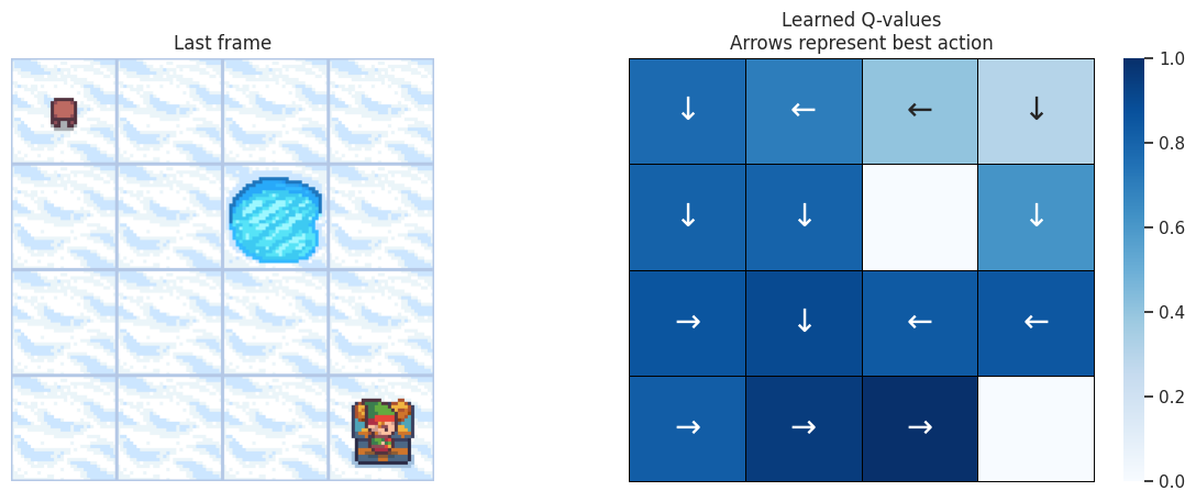
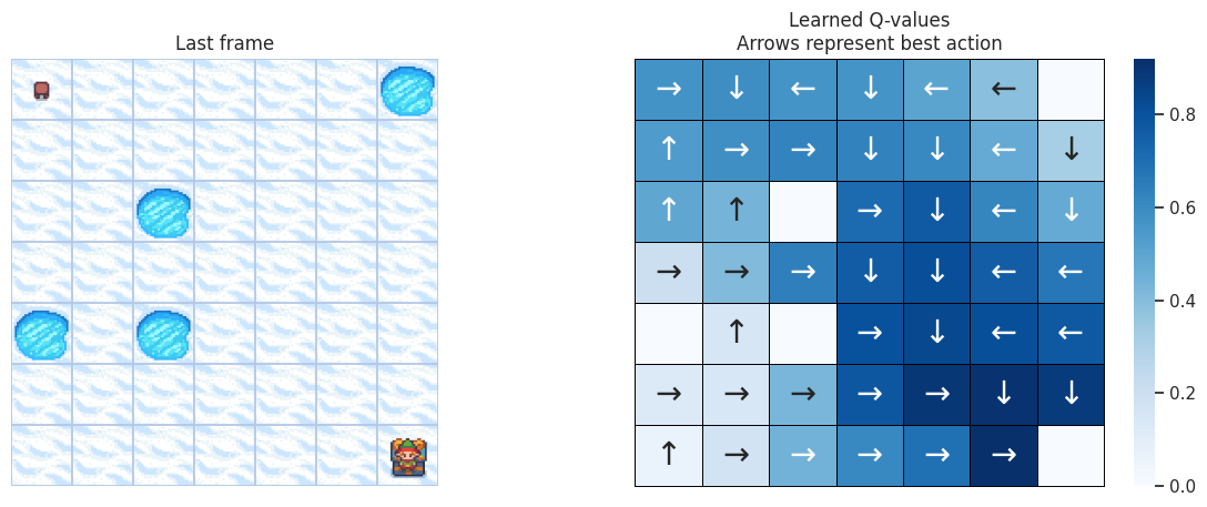
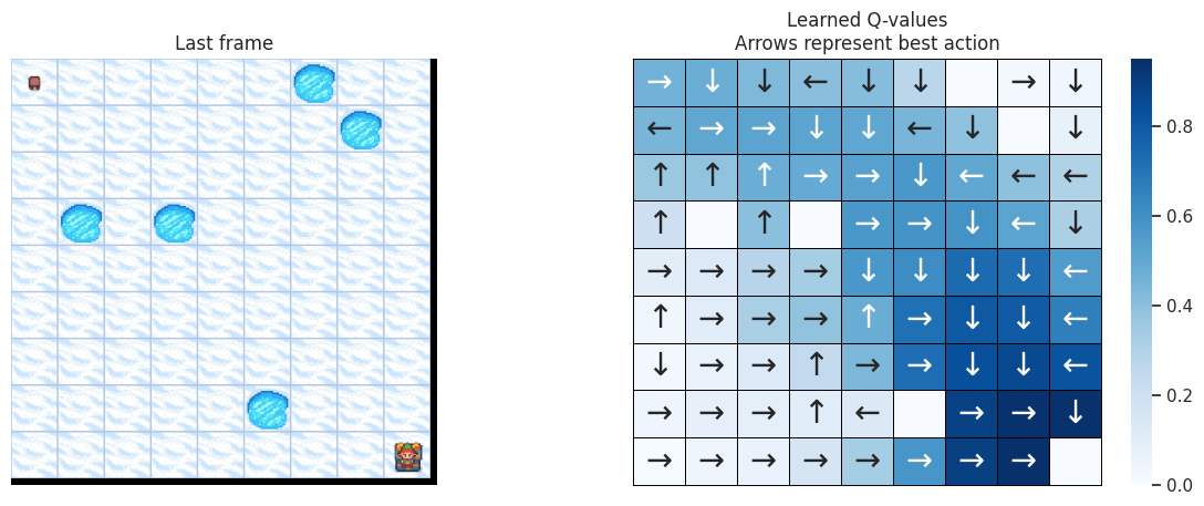
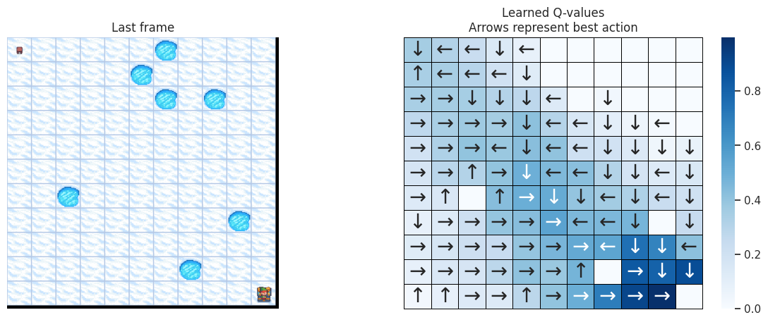
使用以下函式,我們將在左側繪製模擬的最後一幀。如果智慧體學會了一個好的策略來解決任務,我們期望在影片的最後一幀中看到它位於寶藏的方塊上。在右側,我們將繪製智慧體學習到的策略。每個箭頭將代表每個方塊/狀態應選擇的最佳動作。
def plot_q_values_map(qtable, env, map_size):
    """Plot the last frame of the simulation and the policy learned."""
    qtable_val_max, qtable_directions = qtable_directions_map(qtable, map_size)

    # Plot the last frame
    fig, ax = plt.subplots(nrows=1, ncols=2, figsize=(15, 5))
    ax[0].imshow(env.render())
    ax[0].axis("off")
    ax[0].set_title("Last frame")

    # Plot the policy
    sns.heatmap(
        qtable_val_max,
        annot=qtable_directions,
        fmt="",
        ax=ax[1],
        cmap=sns.color_palette("Blues", as_cmap=True),
        linewidths=0.7,
        linecolor="black",
        xticklabels=[],
        yticklabels=[],
        annot_kws={"fontsize": "xx-large"},
    ).set(title="Learned Q-values\nArrows represent best action")
    for _, spine in ax[1].spines.items():
        spine.set_visible(True)
        spine.set_linewidth(0.7)
        spine.set_color("black")
    plt.show()
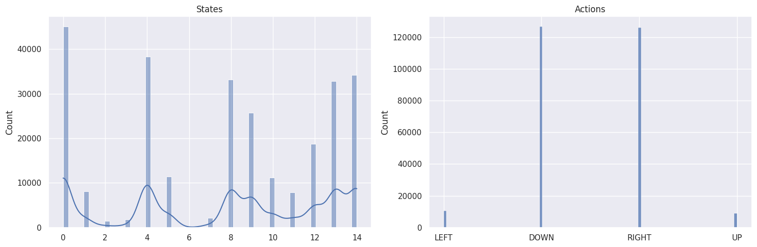
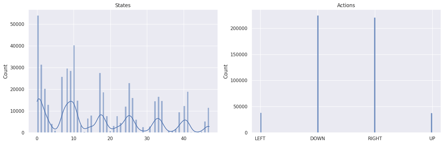
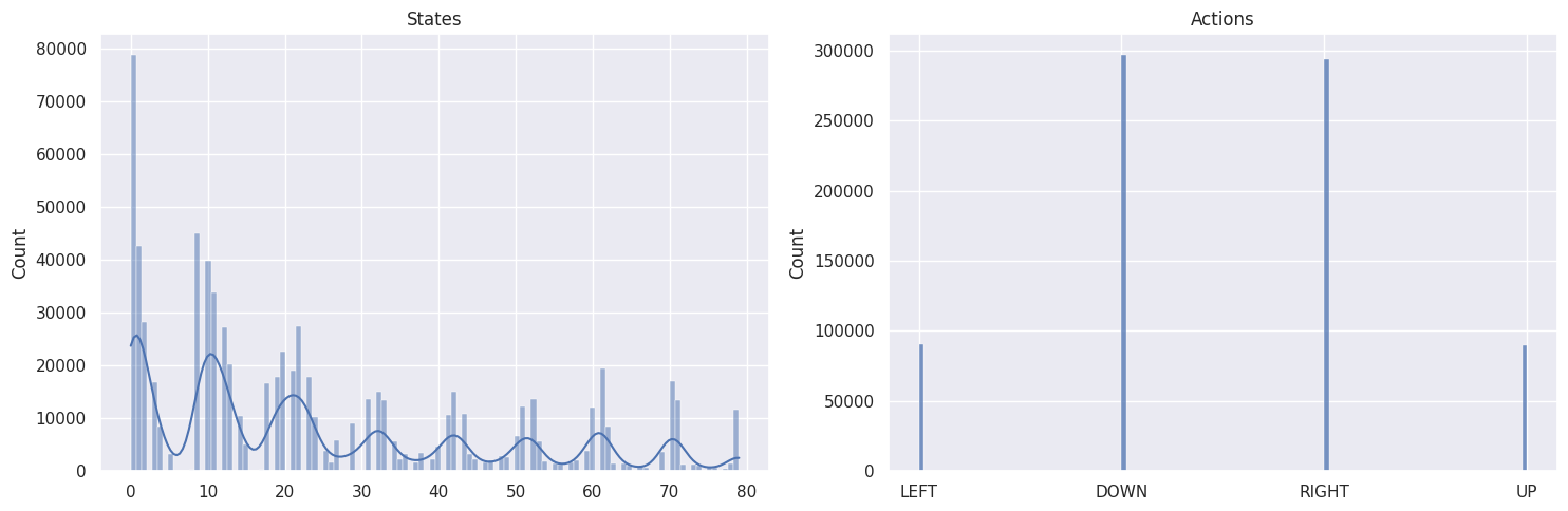
作為健全性檢查,我們將使用以下函式繪製狀態和動作的分佈。
def plot_states_actions_distribution(states, actions, map_size):
    """Plot the distributions of states and actions."""
    labels = {"LEFT": 0, "DOWN": 1, "RIGHT": 2, "UP": 3}

    fig, ax = plt.subplots(nrows=1, ncols=2, figsize=(15, 5))
    sns.histplot(data=states, ax=ax[0], kde=True)
    ax[0].set_title("States")
    sns.histplot(data=actions, ax=ax[1])
    ax[1].set_xticks(list(labels.values()), labels=labels.keys())
    ax[1].set_title("Actions")
    fig.tight_layout()
    plt.show()
現在我們將在幾個不斷增大的地圖尺寸上執行我們的智慧體:- \(4 \times 4\),- \(7 \times 7\),- \(9 \times 9\),- \(11 \times 11\)。
整合所有
map_sizes = [4, 7, 9, 11]
res_all = pd.DataFrame()
st_all = pd.DataFrame()

for map_size in map_sizes:
    env = gym.make(
        "FrozenLake-v1",
        is_slippery=params.is_slippery,
        render_mode="rgb_array",
        desc=generate_random_map(
            size=map_size, p=params.proba_frozen, seed=params.seed
        ),
    )

    params = params._replace(action_size=env.action_space.n)
    params = params._replace(state_size=env.observation_space.n)
    env.action_space.seed(
        params.seed
    )  # Set the seed to get reproducible results when sampling the action space
    learner = Qlearning(
        learning_rate=params.learning_rate,
        gamma=params.gamma,
        state_size=params.state_size,
        action_size=params.action_size,
    )
    explorer = EpsilonGreedy(
        epsilon=params.epsilon,
    )

    print(f"Map size: {map_size}x{map_size}")
    rewards, steps, episodes, qtables, all_states, all_actions = run_env()

    # Save the results in dataframes
    res, st = postprocess(episodes, params, rewards, steps, map_size)
    res_all = pd.concat([res_all, res])
    st_all = pd.concat([st_all, st])
    qtable = qtables.mean(axis=0)  # Average the Q-table between runs

    plot_states_actions_distribution(
        states=all_states, actions=all_actions, map_size=map_size
    )  # Sanity check
    plot_q_values_map(qtable, env, map_size)

    env.close()
地圖尺寸:\(4 \times 4\)
地圖尺寸:\(7 \times 7\)
地圖尺寸:\(9 \times 9\)
地圖尺寸:\(11 \times 11\)
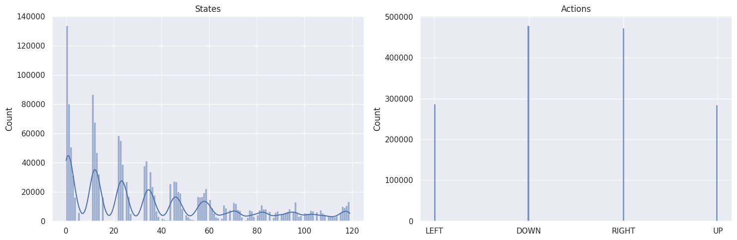
DOWN 和 RIGHT 動作被選擇的次數更多,這很有道理,因為智慧體從地圖的左上角開始,需要找到通往右下角的路徑。此外,地圖越大,離起始狀態越遠的狀態/方塊被訪問的就越少。
為了檢查我們的智慧體是否正在學習,我們希望繪製獎勵的累積和,以及完成劇集所需的步數。如果我們的智慧體正在學習,我們期望看到累積獎勵增加,而解決任務所需的步數減少。
def plot_steps_and_rewards(rewards_df, steps_df):
    """Plot the steps and rewards from dataframes."""
    fig, ax = plt.subplots(nrows=1, ncols=2, figsize=(15, 5))
    sns.lineplot(
        data=rewards_df, x="Episodes", y="cum_rewards", hue="map_size", ax=ax[0]
    )
    ax[0].set(ylabel="Cumulated rewards")

    sns.lineplot(data=steps_df, x="Episodes", y="Steps", hue="map_size", ax=ax[1])
    ax[1].set(ylabel="Averaged steps number")

    for axi in ax:
        axi.legend(title="map size")
    fig.tight_layout()
    plt.show()


plot_steps_and_rewards(res_all, st_all)
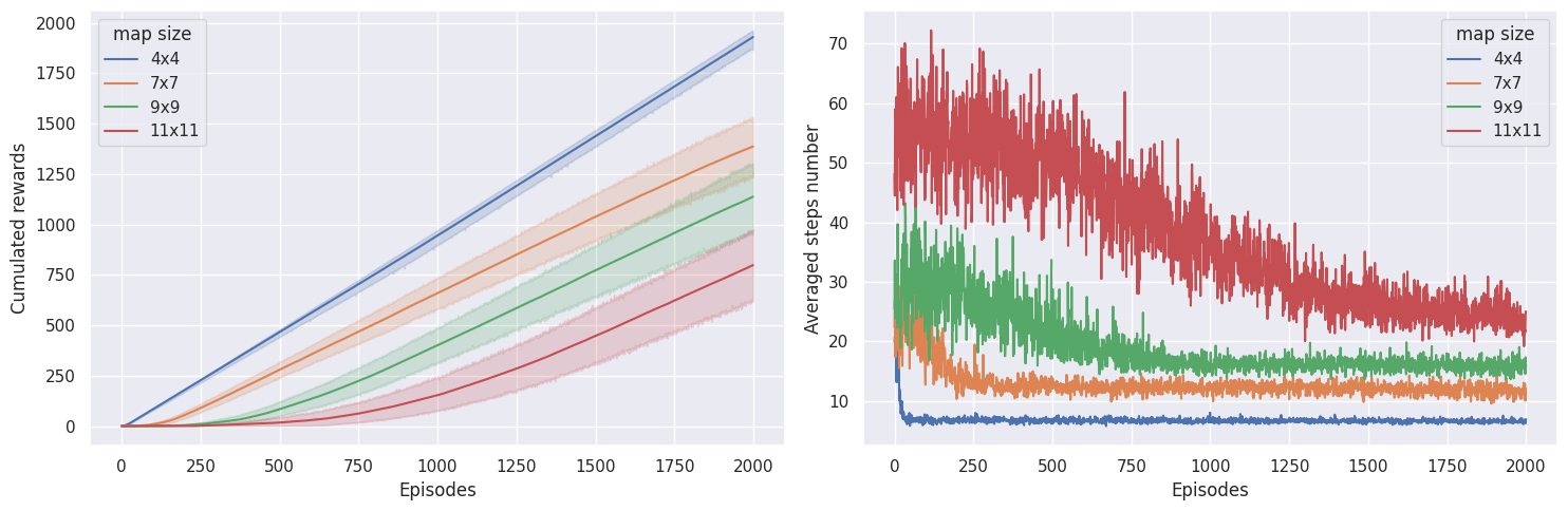
在\(4 \times 4\)地圖上,學習收斂得非常快;而在\(7 \times 7\)地圖上,智慧體需要約\(\sim 300\)個劇集;在\(9 \times 9\)地圖上,需要約\(\sim 800\)個劇集;在\(11 \times 11\)地圖上,則需要約\(\sim 1800\)個劇集才能收斂。有趣的是,智慧體在\(9 \times 9\)地圖上獲得的獎勵似乎比在\(7 \times 7\)地圖上更多,這可能意味著它在\(7 \times 7\)地圖上沒有達到最優策略。
最終,如果智慧體沒有獲得任何獎勵,獎勵就不會傳播到Q值中,智慧體也就學不到任何東西。根據我在此環境中使用\(\epsilon\)-貪婪策略和這些超引數及環境設定的經驗,地圖尺寸大於\(11 \times 11\)的方塊開始變得難以解決。也許使用不同的探索演算法可以克服這一點。另一個影響很大的引數是proba_frozen,即方塊結冰的機率。如果冰洞太多,即\(p<0.9\),Q學習將很難避免掉入冰洞並獲取獎勵訊號。
參考文獻
程式碼靈感來自 Thomas Simonini 的 深度強化學習課程 (http://simoninithomas.com/)
David Silver的課程,特別是第4課和第5課
Q-學習:離策略TD控制,出自《強化學習:導論》,作者Richard S. Sutton和Andrew G. Barto
Tim Miller(墨爾本大學)的強化學習導論